Multinomial Naive Bayes Classifier
Though it’s naive, Naive Bayes classifier is a powerful algorithm commonly used for text classifying. This post has two parts. The first part discusses the Multinomial Bayes classifier and How the algorithm works. Part two is the implementation of the Multinomial Naive Bayes classifier from scratch. Check part two here.
Multinomial Naive Bayes algorithm is a probabilistic learning method that is mostly used in Natural Language Processing (NLP). A simple example for Multinomial Bayes classifier is a spam filter. It classifies the message as spam or not spam. What makes the Naive naive is that it understands a text as a composition of words without considering its structure or context. That means it assumes there is no difference between the texts “A man kills a snake” and “The snake kills a man” because their composition is the same.
Our interest in the Naive byes classifier is to find the probability of a document being in a specific class given that the document is composed of some words. It uses the Bayes theorem to solve this which is given as follows.
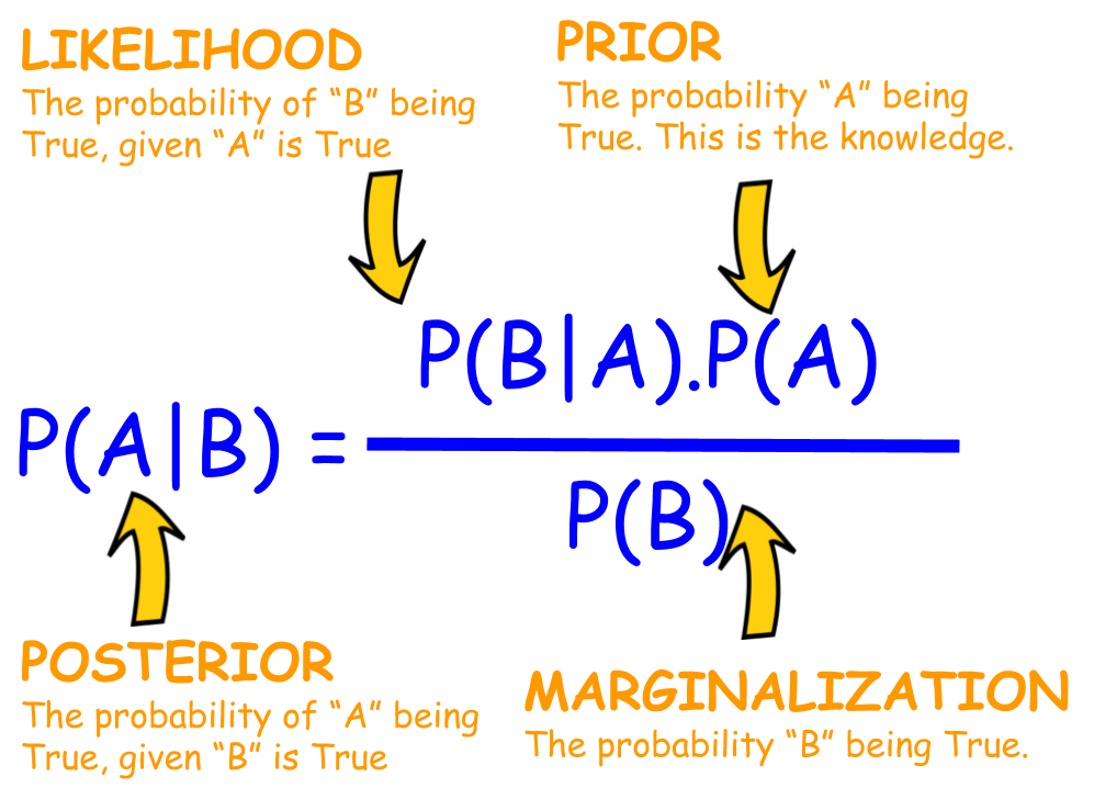
For our case the Bayes theorem becomes
Where ${P(S|w_{1},w_{2},w_{3}...w_{n})}$ is the probalblity of the document being spam given its words are ${w_{1},w_{2},w_{3}...w_{n}}$ . Assuming independency this can be written as
${P(S|w_{1},w_{2},w_{3}...w_{n})=P(S|w_{1})\cdot P(S|w_{2}) \cdot P(S|w_{3})...P(S|w_{n})}$
${P(S|w_{1},w_{2},w_{3}...w_{n})=\frac{P(w_{1}|S)\cdot P(w_{2}|S) \cdot P(w_{3}|S) ... P(w_{n}|S) \cdot P(S)}{P(w_{1}) \cdot P(w_{2}) \cdot P(w_{3})...P(w_{n})}}$
${P(w_{1}) \cdot P(w_{2}) \cdot P(w_{3})...P(w_{n})}$ is constant for every document in the documents we have. We can remove it, since it's like a scaling factor that doesn't change anything in the learning.
${P(S|w_{1},w_{2},w_{3}...w_{n}) {\propto} P(w_{1}|S)\cdot P(w_{2}|S) \cdot P(w_{3}|S) ... P(w_{n}|S) \cdot P(S)}$
This can be written as:
${P(S|W) {\propto} \prod_{i=1}^n P(w_i|S) \cdot P(S)}$
We left with something compact. ${P(S)}$ is the prior probability which is an initial guess about the message is spam. This can be taken the number of messages labeled as spam among the total messages. For example, if we have 600 spam messages among 1000 messages the prior probability would be 0.6. That means initially we roughly guess that every message to be predicted is 60% likely spam.
${P(w_i|S)}$ is the likelihood probability. This is where the effect of each word comes into account. Our initial guess(the prior) will be updated based on this probability. ${P(w_i|S)}$ is the probability of seeing a word ${w_i}$ give that it was in a spam message. This can be computed as the total number of times a word found in spam messages divided by the total number words in spam messages. For example, If we have the word 'money' 250 times repeated in the spam messages and the number of words in the spam messages is 1000 ${P(money|S)}$ becomes 250/1000=0.25.
${P(S|W)}$ is the posterior probability where ${W}$ is the set of the words in the document. The posterior probability is what we would like to find out which is the probability of the message being spam given that its words are ${W}$. In other words, we are trying to find how much percent we are sure the document is spam.
So far we know the probability of the message being spam but the Multinomial Naive Bayes algorithm is not about finding the 'spamity' of the message. It is classifying the message is spam or not. It is easy! We find the probability of the message is normal in the same we found the probability of the message is spam and we compare the results. If the probability of the message being normal is greater than it is spam then we classify the message as normal and vice-versa. Job done. We can put this as:
${y= argmax([P(S|W),P(N|W)])}$
Where ${y}$ is the label of the class and ${P(N|W)}$ is computed similarly as ${P(S|W)}$:
${P(N|W) {\propto} \prod_{i=1}^n P(w_i|N) \cdot P(N)}$
Before going to the implementation we need to do something to prevent arithmetic underflow that will happen when we do the product of the probabilities above. Probability is a number between 0 and 1, product of many of these numbers result in a very small number. Which may result in underflow. To solve this we take the logarithm of it which results in the addition of the probabilities instead of multiplication.
${\log {(P(N|W))} {\propto} \log{(\prod_{i=1}^n P(w_i|N) \cdot P(N))}}$
${\log {(P(N|W))} {\propto} \sum_{i=1}^n \log{P(w_i|N)} + \log{P(N)}}$
${\log {(P(S|W))} {\propto} \sum_{i=1}^n \log{P(w_i|S)} + \log{P(S)}}$
Here we have seen the multinomial Naive Bayes classifier in a simple spam filter use case which is a binary classification but the principle is the same for multicalssification case. I hope you enjoyed it. Next we'll see the implementation of multinomial Bayes classifier. Check part-2 here.